The goal of this post is to learn about Markov Chain Monte Carlo. What is it, why does it exist, how do we “do it”, and how can we apply it to a real problem?

What is Markov Chain Monte Carlo?

Markov Chain Monte Carlo (MCMC) sounds cool. Maybe you know what Markov chains are and/or maybe you know what Monte Carlo methods are. I was familiar with both, but I had no idea what MCMC is.

In a frustratingly short description - MCMC is a way to approximate an integral. That certainly wasn’t the answer I was expecting when I learned about it. There’s so much more to it than that, but that is essentially the heart of it.

But what is it really? Where does it get its name from? Why does it pop up in statistics? To understand that, we’ll need to understand a few things first. So I’ll try to describe it, and then we can work through the explanations that hopefully get us to understanding the description.

MCMC is a way of estimating an intractable integral. It turns out that this is very useful for sampling from distributions in Bayesian statistics. Its name comes from the fact that it uses Monte Carlo sampling to estimate an integral, and the process for generating the Monte Carlo samples is actually a Markov chain.

But I didn’t really know what that meant at first.

• What makes an integral intractable?
• Why is estimating an integral useful in Bayesian statistics?
• What even is Bayesian statistics; how is it meaningfully different from general “statistics”?
• Why is sampling from a distribution difficult?

What makes an integral intractable?

Well, there’s sort of two, overloaded definitions here:

1. the integral cannot be solved analytically
2. the integral cannot be computed in closed form (i.e it involves some infinite summation)

If the integral could be solved analytically, we wouldn’t need extensive computation. If it’s not analytically solvable and it involves some infinite summation, then you can’t compute that finitely. So you need to approximate the integral. There are other ways of approximating this integral, but MCMC is one of the more efficient ways, especially in higher dimensions. (TODO - elaborate on why it’s more efficient)

Why is estimating integrals useful in Bayesian statistics?

A quick aside about Bayesian stats and inference

I was familiar with Bayes’ formula, but I don’t think I appreciated the meaning of the equation in the context of MCMC originally.

Where \(H\) is our hypothesis and \(D\) is our data. Basically this is saying, if you have some prior hypothesis \(H\), you can make a better, updated hypothesis (the posterior) once you’ve seen some data \(D\).

When I describe Bayesian inference to some friends, their eyes glaze over. Writing the formula down is one thing, but trying to describe it verbally is an awful mouthful. I think it’s helpful to point out that we all do Bayesian inference all the time - just without realizing it necessarily. For anyone that’s played competitive sports, we typically use such inference. For example, say you’re a defender in soccer. You know that like 90% of people are right-footed. So by default, when you play against someone new, you’re going to defend them as if they’re right-footed: force them onto their left etc. But say you’re playing against someone one day, and you notice that they’re dribbling against you with their left foot. You don’t know for sure, but there’s a better chance than usual that they’re left-footed. As the game progresses, and they continue to favor their left foot, you become more confident that they’re left-footed. This is essentially Bayesian inference. In general, we know from experience that most people are right-footed. But in this particular case, now that we’ve collected data from our opponent, we have reason to believe that they’re actually left-footed.

I think the wiki article on Bayesian inference does a good job of describing the symbols here.

So why is MCMC useful?

Basically because integrals appear often in Bayesian statistics. It turns out that actually calculating the posterior invovles an often times intractable integral because of the denominator \(P(D)\).

I was often confused in MCMC explainers because they so often presented MCMC exclusively in context of computing posterior distributions. MCMC is useful for determining a posterior distribution, but it’s not used exclusively for that. MCMC is useful for estimating an integral. It turns out that we need to do just that when determining a posterior distribution. A posterior distribution is basically just fitting a model to data, kind of like how we fit a linear regression model to data.

So MCMC can do two things for us. First, it helps us avoid calculating \(P(D)\) directly, which allows us to get \(P(H \mid D)\) more easily. Second, it allows us to sample from \(P(H \mid D)\) as well.

To appreciate the second point, it’s important to understand that sampling from a distribution is non-trivial.

How would you sample from a uniform distribution? What about a normal distribution?

Why is sampling from a distribution difficult?

• uniform distro: Mersenne twister or linear feedback (simplest)
• normal distro
• general distro

How and why does MCMC work?

So now we know why we want MCMC. We have a model and we have some data. We want to fit the model to the data. We are obstructed by the difficulty in computing \(P(D)\), the evidence.

Quick aside

One of the things that initially frustrated me about MCMC came from my misunderstanding what MCMC actually does. I naively thought it was just a way of getting “some” model to arise for your data. But MCMC is a way to fit a parametric model to data. MCMC requires you to specify a model with parameters, and then you’re only adjusting those parameters. Those parameters themselves can be modeled as distributions. I was confused when the blogs would do all this work and then finish with a plot of the posterior model for the parameters, instead of for the data. But it’s important to realize that if you have a posterior for your parameters, then you have a posterior for your data as well! Since your data model is defined entirely by those parameters.

Note that if we ignore the evidence component, then we at least have a function that is proportional to our desired posterior distribution.

So essentially \(\dfrac{1}{P(D)}\) normalizes \(P(D \mid H)P(H)\) so that we get a well behaved PDF.

Even though we don’t know how to compute our posterior, we do know that it exists. Our goal then is to construct a Markov chain with a stationary distribution equal to our desired posterior distribution. If we can do this, then we can run the Markov chain for a long time, and it will essentially be like sampling from the posterior.

The Markov chain we’re creating has a continuous state space over \(\mu\) and \(\sigma\). We need to define a transition function such that repeated iterations of the process converge to the posterior \(P(H \mid D) = CP(D \mid H)P(H)\) where \(C\) is some normalizing constant.

We can choose an arbitrary initial state \((\mu_0,\sigma_0)\). We propose some new state \(p = (\mu_p,\sigma_p)\). The probability that we accept \(p\) should be equal to the posterior. We could maybe transition to it with probability \(min(1, P(D \mid p)P(p))\) but what about \(C\)?

It’s useful to note the relative likelihood of observing certain samples from a distribution. It’s easier to highlight with a discrete distribution. Imagine we know the distribution of favorite number between 1 and 10. Say 7 is extremely popular, with 50% of people saying it’s their favorite. 6 on the other hand is very unpopular, with only 5% of the population saying it’s their favorite. We should expect to see 7 ten times as often as we see 6.

We can do something similar for our posterior distribution. If we have two samples \(p_1\) and \(p_2\), then

This is great! We now have a function to describe \(P(H \mid D)\) that avoids \(P(D)\) entirely and is described by two possible samples.

So going back to our Markov chain, we can try to construct the transition function to be equal to \(\dfrac{P(D \mid p)P(p)}{P(D \mid p_c)P(p_c)}\)

This is readily doable if we define the probability of transitioning to state \(p\) as \(min(1, \dfrac{P(D \mid p)P(p)}{P(D \mid p_c)P(p_c)})\).

For this to be useful, we want to propose reasonable \(p\) values. We could maybe sample uniformly from some finite space. Or, as we’ll do in this post, we can sample from a normal distribution centered at the current value, \(p_c\). This is more efficient because if we’re sampling uniformly, we’ll get any random value which not be good, so we’d end up rejecting lots of samples. Instead, if we sample near \(p_c\) the new proposed value \(p\) should be relatively similar in likelihood, and therefore more likely to be accepted.

A real world example

I struggled to understand many of the blogs I read because they didn’t use an example. So I hope to illustrate MCMC using a concrete example. That said, I found this blog to do a pretty good job of explaining the algorithm.

Let’s say we want to model daily SPY returns. I actually did a first draft of this that tried to model them as a normal distribution. The results were lackluster. I’d normally include them for transparency sake, but in the interest of brevity, I’m excluding them. The point is that I tried one type of model first, didn’t like it, and tried again with a second model.

So we’re going to model the returns as a t-distribution. To be honest, I don’t know if this is bad practice, since I think t-distributions are meant to be stand-ins for normal distributions when you don’t have a lot of data.

We don’t have any data to look at right now, but we have some rough assumptions about how markets work, so let’s go from there: we could say the mean \(\mu\) is 0 and the standard deviation \(\sigma\) is 0.01 - or, in other words, 1%. t-distributions also have a degrees-of-freedom (DF) parameter, but I’m less interested in fitting that for now (you can feel free too, I’m just taking a lazy shortcut). Let’s say DF=20.

But let’s be a bit more realistic. We definitely don’t know the best values for \(\mu\) and \(\sigma\). Why should we pretend that we do by choosing a single value for each? Instead, let’s admit uncertainty and instead describe \(\mu\) and \(\sigma\) probabilistically.

For \(mu\), we can model it as a normal distribution. For \(sigma\), since it’s non-negative, we can model is as a half-normal distribution. We’ll try to choose reasonable parameters for these, but again, these are prior models, so there’s a good chance our choices will be bad.

So we have

Once we fit it with data and generate a posterior, we’ll have a better model. And that’s the whole point, after all.

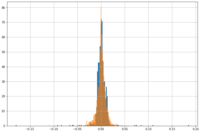
So let’s say we’ve collected data. We have the daily returns for SPY going back the last 10 years. I’d like to plot the data histogram next to our prior model as a visual sanity check of how far off we are.

The thing is though that our model is hierarchical, so it’s not trivial to draw it like we would with a normal curve. We could just use single values for the parameters, but that’s misleading. Instead we can sample from our prior and plot that histogram for comparsion.

We sample from our prior by repeatedly sampling \(\mu\) and \(\sigma\) from their distributions, plugging those in as single values for the data model, and then sampling from that distribution.

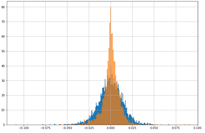
Orange is the data and blue is our model. We can see clearly that our model doesn’t align very well.

So now we can start computing our posterior.

So we want \(P(D \mid H)P(H)\). Even as I was writing this, I kind of got confused: wait, what does \(P(H)\) even mean? How do we calculate that? Well, our hypothesis/model is parameterized by two variables: \(\mu\) and \(\sigma\). We said earlier that for our prior model, we were modeling \(\mu\) and \(\sigma\) each as normally distributed. So we can rewrite \(P(H)\) as \(P(\mu,\sigma)\) which is basically the joint probability of our two variables: for a given pair \((\mu,\sigma)\), how likely is that pair explainable by our prior model for the parameters?

We said that computing \(P(D)\) is too difficult. Instead we’ll get at our posterior by using rejection sampling.

The sampling is pretty straightforward (for our example; there are more sophisticated sampling methods).

We will basically be generating a stream of numbers from two normal distributions for \(\mu\) and \(\sigma\).

Quick aside

I want to make a note here because I got confused about this many times. The distributions here for picking new proposal values for \(\mu\) and \(\sigma\) have nothing to do with the distributions we’ve already mentioned. So we now have mentioned three different sets of distributions that are different:

• the model for our data
• the model for the parameters of our data model
• how we want to pick new proposal values for \(\mu\) and \(\sigma\)

For each of the proposed number pairs, we compute the likelihood function using this pair as the new \(\mu\) and \(\sigma\). We then compare this likelihood to the likelihood of the previously accepted \(\mu\) and \(\sigma\). If the proposal is better, we accept it. If it’s worse, we accept it with probability \(\dfrac{P(D \mid \mu_{p},\sigma_{p})}{P(D \mid \mu_{c},\sigma_{c})}\). If we reject it, we simply don’t have a new sample yet, and will try again. So theoretically if you choose a very bad way of picking proposals, it could take you a longer time to generate samples.

This entire algorithm can fit into a short python program:

def likelihood(u,g, data):
    """
    the algorithm here is incorrect b/c it adds the pdf values instead of multiplying them,
    but I found using log probability or multiplication led to unstable results
    """
    acc = 1
    for x in stats.t.pdf(data, df=50, loc=u, scale=g):
        if not np.isnan(x):
            acc += x
    return acc
 
def prior(u, g):
    u_p = stats.norm(0.001, 0.01).pdf(u)
    g_p = stats.halfnorm(0, 0.001).pdf(g)
    return u_p * g_p

def sample(u_c, g_c):
    likelihood_current = likelihood(u_c, g_c, spy['%Return'])
    prob_current = likelihood_current * prior(u_c, g_c)

    u_p = np.random.normal(u_c, 0.001)
    g_p = np.random.normal(g_c, 0.001)

    likelihood_p = likelihood(u_p, g_p, spy['%Return'])
    prob_p = likelihood_p * prior(u_p, g_p)
    r = np.random.uniform()
    if r < prob_p / prob_current:
        return u_p, g_p
        
    return None 

u = 0.001
g = 0.01
i = 0
likelihood_current = likelihood(u, g, spy['%Return'])
prob_current = likelihood_current * prior(u, g)
samples = [(u, g)]
while i < 10000:
    if i % 1000 == 0:
        print(f'{i}th step', len(samples))
    i += 1
    theta = sample(u, g)
    if theta is None:
        continue
    u,g = theta
    samples.append((u,g))

Here are the results I got from running this code:

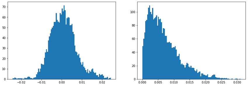
These are the histograms of the sampled posterior values for \(\mu\) and \(\sigma\).

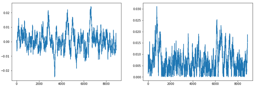
These are the traces for \(\mu\) and \(\sigma\). This is just plotting how the current \(\mu\) and \(\sigma\) are changing over time. It’s good for a sanity check to ensure our samples have converged and are also not overly autocorrelated.

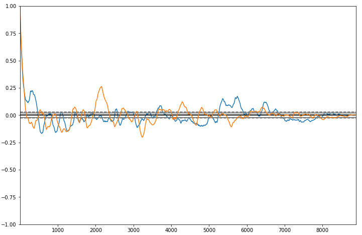
These are the auto-correlation graphs for \(\mu\) (orange) and \(\sigma\) (blue).

Doing it by hand

We can work through the first iteration as an exercise. We’ve chosen initial values for \(\mu\) and \(\sigma\) as 0.001 and 0.003. These values can be arbitrary. If you choose something ridiculuous, it’ll take longer to converge.

Then, we choose a random proposal value for each of \(\mu\) and \(\sigma\). Like I said earlier, we use a normal distribution to sample from, but we could use many other samplings methods as well. Technically speaking, the choice of method does matter because we care about reducing autocorrelation between our samples. Ideally, we could sample from our distribution independently, but this form of rejection sampling is after all a Markov chain, which means there will be some dependence on the previous value. If you choose a poor method, you might observe higher autocorrelation.

Say the first proposal value is (0.005, 0.008). Then we’d compute the likelihood function for this pair, multiply by the probability of this pair coming from our prior model for \(\mu\) and \(\sigma\), and then compare to the same computation for our initial pair.

So say we generate a random number between 0 and 1 that is less than 0.599. We’d accept this new pair (0.005,0.008) and repeat the process using this one as the current sample.

We do this for a long time until we’ve generated many samples. We’ll want to discard some of the early samples because of this thing called burn-in. Basically, since our samples are auto-correlated and our initial pick probably isn’t super close to the best pick, it means that the first several samples will be biased towards our initial pick. If you’re familiar with Markov chains, this is basically just saying that it takes some iterations to converge to the stationary distribution.

So now we have a new model for \(\mu\) and \(\sigma\), which essentially means that we have a new model for our data.

I was initially frustrated when I saw many of the explainers I was reading conclude with plots of the parameter posteriors. I want to simulate data, not parameters! And honestly, it’s not exactly trivial to generate fake data. It is if you know what you’re doing, but I didn’t!

The key insight is that you’re interested in the posterior predictive distribution \(P(D* \mid D)\) which we can get by continuing to sample parameters \(\theta\) and for each \(\theta_i\), draw \(D* ~ P(D | \theta_i)\). How do we draw that though? Well, we actually just plug in the parameter values from \(\theta_i\) into our data model and sample from that.

That looks a lot better!

But as I said above, this wasn’t the first run. My normal model results were lackluster, and I also played with the prior parameters a bit before the fit looked this good. I found from doing this exercise that the prior matters more than I would’ve thought.

Also, it’s possible that modeling returns like this as a symmetric t-distribution is inherently flawed. We could try MCMC with a more complicated model, or we could try using non-parametric estimation. I will try to cover that in another post soon.