I recently realized that I didn’t understand linear regression as well as I thought as I did when I came across this twitter thread.

Okay, I thought, so maybe I don’t know exactly how to do it with linear algebra but I intuitively know how to draw a best fit for a set of points, so I should be able to work from there and develop a more rigorous algorithm of what I’m doing by intuition.

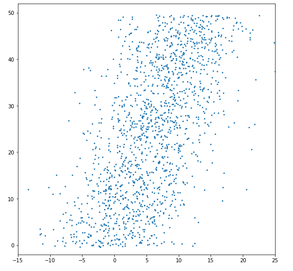
For example, for this set of points, what line would you draw?

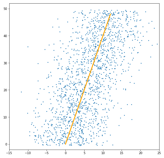
I’d draw a line looking like this

Except that’s not correct if you’re using least squares. This is the correct fit.

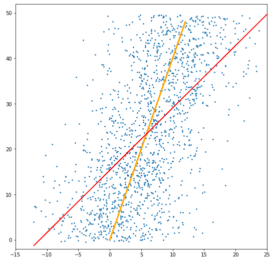
Oh. Oops. Looks like I need to learn linear regression beyond just importing scikit-learn.

_{^{What went wrong? I drew the line which minimizes the euclidean distance between the points and the line, but that’s not actually useful for prediction (in typical cases). That’s because if I’m given an input, I want to guess the output for that input. We’re given the X value, so we’re not trying to change anything related to that. But when we do the euclidean distance minimization, then you do change the X value. So that’s kind of silly (again, in typical cases). So since we want to only change the Y value, that means we’re changing the vertical value of the point, or in other words, minimizing the vertical distance. Which ends up being the least squares formula.}}

It’s pretty easy to google for basic blog posts about linear regression, so why am I writing another one? Well, for one, it’s helping me to consolidate my learnings into notes. But also, I found the blogs to be unsatisfactory in giving me a deep understanding. I didn’t just want to see how to solve the least squares problem, I wanted to know why the “how” worked.

I’ll try to cite the blogs and stackexchange posts that I came across and relied on as I built up my understanding. I’ve also included them at the end.

_{^{The tweet only says “least squares problem”, which might refer to a more general problem, but I’m going to focus on just the linear least squares problem for simplicity purposes.}}

It seems like there are two approaches to solving the problem. One approach defines a cost function that describes how good/bad the model is, and then minimizes that cost function. The other approach uses linear algebra to project the data onto a line. This is the one I struggled to develop an intuition for, because the approach never explicitly uses a cost function or derivative, so it wasn’t clear to me how a solution could just “emerge”.

I view the two approaches as having different equations. The calculus approach is solving \(A\hat{b} \approx Y\) by trying to find some \(\hat{b}\) that gets us close to a good solution. The linear algebra approach is solving \(Ab = \hat{Y}\) where we give up on solving \(Ab = Y\) which is likely impossible, and instead solving a similar problem where we move all the points onto a hypothetical line.

Calculus approach

So we have all these data points. We can rewrite them as a system of linear equations. And rewrite that in matrix notation: \(Ab = Y\). There almost definitely does not exist any \(b\) that satisfies this equation. So the best we can do is some approximation: \(A\hat{b} \approx Y\) How do we define a best approximation? We need some way to compare different possible values for \(\hat{b}\). So we define a cost function that describes how far off our solution is from reality, and seek to minimize this function.

A popular choice of cost function is least squares: \(S = \sum_{i}^{N}(y_{i} - \hat{y_{i}})^2\). As for why least squares is a popular choice, this stackexchange post does a good job of explaining. For starters, it’s probably the simplest reasonable cost function to calculate. But I also learned from writing this blog that there’s a pretty beautiful relation between least squares and the smallest distance between \(Y\) and \(\hat{Y}\) when you consider them as vectors in N-dimensional space (where N is the number of data points we have). I cover that a little bit in the linear algebra approach section.

We can rewrite our cost function as \(\sum_{i=1}^{N} (y_{i} - \hat{y_{i}})^2 = \sum_{i=1}^{N} (y_{i} - b * x_{i})^2\).

We wish to minimize it with respect to the input coefficients. For which we have just one for now.

To minimize, we want to find where its derivative is 0: \(dS = \sum_{i=1}^{N} -2x_{i} * (y_{i} - b * x_{i}) = 0\)

Then it is a matter of reducing the equation:

1. separate: \(\sum_{i=1}^{N} x_{i} * y_{i} - \sum_{i=1}^{N} b * x_{i}^2 = 0\)
2. \[\sum_{i=1}^{N} x_{i} * y_{i} = \sum_{i=1}^{N} b * x_{i}^2\]
3. \[\sum_{i=1}^{N} x_{i} * y_{i} = b * \sum_{i=1}^{N} x_{i}^2\]
4. \[b = \dfrac{\sum_{i=1}^{N} x_{i} * y_{i}}{\sum_{i=1}^{N} x_{i}^2}\]

If we had more coefficients, then we’d no longer be deriving along just one dimension. We’d need to write out the partial derivatives with respect to each of the coefficients to build the gradient. If we have \(k\) coefficients, then the best line would be described as a point in k-space where the gradient is zero for all of the coefficients. We can guarantee that such a point exists because our least squares cost function is strictly convex, meaning that if a line is drawn between any two points on the curve, all points on the line lie above the curve. This is because the least squares function is a paraboloid function. The implication of it being strictly convex means there’s no local up-and-downs, so there has to be a unique global minimum.

Linear algebra approach

Like I said, I struggled to intuitively understand this approach. Defining a cost function and minimizing it made sense to me. You can start with a terrible fit and optimize it. But I couldn’t understand how you could just “get” the optimal solution in a closed form formula that didn’t involve any derivatives (or even the cost function!). This post was the first one I looked at that introduced the linear algebra solution. Even though the logic is sound, I found myself confused because I feel that it glosses over important steps.

Part of the reason I’m emphasizing the why of this approach so much is that in order to make sense of \(Ab = \hat{Y}\), I visualized it as moving all our data points so that they fit some hypothetical line perfectly. This is a geometric interpretation so I wanted to be able to draw some kind of isomorphism between all the linear algebra operations and some geometric interpretation so that ultimately, I could see how there’s meaning in the way we move the data points.

So let’s go back to the points we had above. We’re solving a 2-dimensional linear regression. So you have all your points e.g (1,3), (1,5), (2,3), (3,4), (3,6), (3,7), …, (10,6), (10,11), (10,12). Since we’re ultimately trying to find a single linear solution (of the form \(y = cx + b\)) that fits these points, you can rewrite your points as a system of linear equations.

\[x=3\\x=5\\2x=3\\3x=4\\...\]

And we can straightforwardly rewrite this in matrix notation as

\[\begin{bmatrix}1\\1\\2\\3\\3\\3\\...\\10\\10\\10\end{bmatrix} \begin{bmatrix}x\end{bmatrix} = \begin{bmatrix}3\\5\\3\\4\\6\\7\\...\\6\\11\\12\end{bmatrix}\]

We’ll label the matrices and rewrite the equation as

\[Ab = Y\]

where we’re trying to solve for \(b\).

Quick note: if we were working with higher dimension data, \(A\) and \(Y\) would have more columns. But we don’t have to worry about that for now since our notation is valid for all dimensions.

Now of course, if you actually tried to solve this solution, you wouldn’t be able to. This is because \(Y\) isn’t in the column space of \(A\) (referred to as \(C(A)\).

I needed a reminder for what a column space was, so I’ll include one here. If you don’t need it, feel free to skip ahead to the next paragraph.

The column space of a matrix \(A\) is essentially the range of the matrix, analogous to the range of a function. It describes the space of all possible linear combinations of the columns of \(A\). Since our matrix has just one column, its column space is actually just a line. If it had two columns, the column space would span a plane. But a line where? Well, say \(A\) has n rows. Then \(C(A)\) would be a line in n-space. So in our case, \(C(A)\) is just a line parallel to the column vector \(A\). Note that \(Y\) is also a vector in n-space. And of course, more likely than not, \(Y\) does not lie on the line \(C(A)\).

So in order to make the problem solvable, we need to project \(Y\) onto \(C(A)\). This is where I got confused when I was learning. The blog examples were often solving a 2D or 3D regression problem, and would also describe \(C(A)\) as a plane. So I assumed that \(C(A)\) was a plane in the same space as the original linear regression problem itself, rather than in the column space. So I kept thinking it meant that for each data point, we needed to somehow project it onto our yet-to-exist solution line/plane. It’s circular reasoning, and also the “projection” here wouldn’t be orthogonal unless the solution line is horizontal. Of course, my thinking didn’t really make sense, but I’m including it here in case someone else is confused because of the different spaces described by the rows and columns. The linear regression problem has the same dimension as the number of columns in \(A\) + 1 for \(Y\). Whereas the column space is concerned with the number of rows / data points in \(A\).

For our example, the projection \(\hat{Y}\) of \(Y\) onto \(C(A)\) is given by:

\[\hat{Y} = \dfrac{Y \cdot A}{A \cdot A}A\]

To visualize why: \(\dfrac{Y \cdot A}{A \cdot A}\) will give us a scalar value. So we’re essentially just computing some extension or contraction of \(A\), which makes sense because \(A\) is our column space when we have just one predictor variable. To understand \(\dfrac{Y \cdot A}{A \cdot A}\) you can picture the two vectors \(Y\) and \(A\). Rotate the picture so that \(A\) is pointing horizontally to the right. Assume for now that \(Y\) also points generally right isntead of left. If you draw a straight line down from the end of \(Y\) to \(A\), that will give you how “long” \(Y\) is “along” \(A\).

Now we can use \(\hat{Y}\) to create a modified equation \(Ab = \hat{Y}\). Which is solvable! We want to isolate \(b\) so we should “divide” by \(A\) on both sides by inverting \(A\). But wait - we can’t invert \(A\) because \(A\) is Nx1 so it’s definitely not invertible. Instead, we can multiply it by its transpose to get a square matrix:

\[A^{T}Ab = A^{T}\hat{Y}\] \[b = (A^{T}A)^{-1}A^{T}\hat{Y}\]

So technically \(A^{T}A\) might not be invertible, but for our practical purposes, we can assume it is because it would require the columns of \(A^{T}A\) to not be linearly independent. I’m unable to prove this in a rigorous way, but you can look at the columns of \(A^{T}A\) and see that they most likely are linearly independent because it’s not clear how to separate out the terms to show an equality with 0. Alternatively, we know the probability of randomly generating a non-invertible matrix is 0, so we can safely assume ours is invertible.

If you’ve read other linear regression explanations, then the above equation probably looks similar, and it’s called the normal equation. My derivation yields different notation than what I’ve seen elsewhere. Some other people use \(\hat{b}\) and \(Y\) to denote a modified solution, but as far as I understand, the equation is only solvable if \(Y\) is projected onto \(C(A)\), so I prefer to show that by using the projection of \(Y\).

We can go another step further. We know \(\hat{Y} = \dfrac{Y \cdot A}{A \cdot A}A\) so we can plug that into the normal equation:

\[b = (A^{T}A)^{-1}A^{T}\dfrac{Y \cdot A}{A \cdot A}A\] \[b = \dfrac{Y \cdot A}{A \cdot A}(A^{T}A)^{-1}A^{T}A\] \[b = \dfrac{Y \cdot A}{A \cdot A}I_{1}\]

So this gives us exactly the coefficient that we want for our regression slope.

But what if we have two or more predictors?

Ideally not much should change, but I did take some shortcuts since we were working in 2d regression. Let’s say we’re working in 3d now.

\(Ab = Y\) still, but now \(A\) is Nx2 instead of Nx1 and \(b\) is 2x1 instead of 1x1.

The column space of \(A\) now spans a 2d plane instead of just a line. So we need to project \(Y\) onto this plane. Before, \(Y\) was simply a contraction or extension of the vector \(A\). But now we have the columns of \(A\) that form a basis for \(C(A)\). Now \(\hat{Y}\) is a linear combination of these basis vectors which will lie somewhere on the plane spanned by \(C(A)\).

We’ll need to generalize the equation we used above in the 2d case:

\[\hat{Y} = \dfrac{Y \cdot A}{A \cdot A}A\]

becomes

\[\hat{Y} = \dfrac{Y \cdot u_1}{u_1 \cdot u_1}u_1 + \dfrac{Y \cdot u_2}{u_2 \cdot u_2}u_2\]

where the vectors \(u_1\) and \(u_2\) form an orthogonal basis for \(C(A)\). ^{This equation also generalizes for any number of dimensions} So essentially \(\hat{Y}\) is a linear combination of vectors that span \(C(A)\).

Unfortunately, if we plug this into the normal equation, we can’t simplify it like we did in the 2d case. Instead we’ll want to use matrix notation to give us terms that we can futher simplify:

\[\hat{Y} = A(A^{T}A)^{-1}A^{T}Y\]

To prove why this is the case would take too much space here. You can read this for a rigorous proof of why that equation is a projection of \(Y\) onto \(C(A)\). Basically, it kind of goes like:

1. \(Y - \hat{Y}\) must be orthogonal to \(C(A)\)
2. Therefore \(Y - \hat{Y}\) is orthogonal to \(Ab\) which is a vector in \(C(A)\)
3. So the dot product \(Ab \cdot (Y - \hat{Y}) = 0\)
4. Rewrite \(Ab\) as \(b \cdot A^T\) so you end up with \(b \cdot (A^{T}(Y - \hat{Y})) = 0\) for all possible vectors \(b\) of size Kx1 where K is the number of columns in \(A\)
5. The only way that’s possible is if \((A^{T}(Y - \hat{Y})) = 0\)
6. Remember that \(\hat{Y} = Ax\) for some \(x\), so \((A^{T}(Y - Ax)) = 0\)
7. Distibute and add: \(A^{T}Y = A^{T}Ax\)
8. Invert: \((A^{T}A)^{-1}A^{T}Y = x\)
9. Multiply both sides by \(A\): \(A(A^{T}A)^{-1}A^{T}Y = Ax = \hat{Y}\)

So even though the proof makes sense to me, I struggled to understand geometrically how/why \(A(A^{T}A)^{-1}A^{T}\) is a projection operator. I think it’s useful to compare what this equation is really doing compared to our original linear combination equation. If we define \(P_{C(A)} = A(A^{T}A)^{-1}A^{T}\) then \(P_{C(A)}Y\) is a linear combination of the columns of \(P_{C(A)}\). If we assume for now that \(A\) is orthonormal, then we can drop \((A^{T}A)^{-1}\). So now we have a linear combination of the columns of \(AA^T\). If we enumerate the row by column multiplication, we’ll see that the columns of \(AA^T\) are themselves linear combinations of the columns of \(A\):

Say

\[A = \begin{bmatrix}a_{11} & a_{12} & ... & a_{1k}\\a_{21} & a_{22} & ... & a_{2k}\\ \vdots \\a_{N1} & a_{N2} & ... & a_{Nk}\end{bmatrix}\]

and

\[A^T = \begin{bmatrix}a_{11} & a_{21} & ... & a_{N1}\\a_{12} & a_{22} & ... & a_{N2}\\ \vdots \\a_{1k} & a_{2k} & ... & a_{Nk}\end{bmatrix}\]

So

\[AA^T = \begin{bmatrix}a_{11}a_{11} + a_{12}a_{12} + ... + a_{1k}a_{1k} & ... & a_{11}a_{N1} + a_{12}a_{N2} + ... + a_{1k}a_{Nk} \\ \vdots \\a_{N1}a_{11} + a_{N2}a_{12} + ... + a_{Nk}a_{1k} & ... & a_{N1}a_{N1} + a_{N2}a_{N2} + ... + a_{Nk}a_{Nk} \end{bmatrix}\]

If \(A\) isn’t orthonormal then we need \((A^{T}A)^{-1}\) to normalize the projection so that it’s orthogonal to \(C(A)\) rather than be at an oblique angle.

So now if we plug \(P_{C(A)}Y\) into the normal equation:

\[Ab = A(A^{T}A)^{-1}A^{T}Y\] \[A^{T}Ab = A^{T}A(A^{T}A)^{-1}A^{T}Y\]

we can cancel the terms:

\[A^{T}Ab = A^{T}Y\] \[b = (A^{T}A)^{-1}A^{T}Y\]

The thing that frustrated me about the other examples online is that they would seem to skip over the projection equation and just derive the normal equation from \(Ab = Y\) (which you can do symbolically), but we know this original equation isn’t solvable. So why is the normal equation solvable? It’s because when you use \(Ab = \hat{Y}\), which is solvable, there are terms that actually cancel out when you isolate \(b\).

What’s the geometric interpretation of this? Well \(Ab = Y\) means we’re hoping to find some linear combination of the column vectors of \(A\) that sum to \(Y\). We know this isn’t possible however. So we instead try to solve for \(Ab = \hat{Y}\) knowing that \(\hat{Y}\) lies in \(C(A)\). If you look at \(Ab = A(A^{T}A)^{-1}A^{T}Y\), this is basically saying that a linear combination of the columns of \(A\) can sum to a projection of \(Y\) onto \(C(A)\). If we could just invert \(A\), it would reduce to our final equation, but we have to take the intermediate step of multiplying it by its transpose to guarantee invertibility.

What about an intercept?

If we want to have an intercept, then our equation looks like \(Ab + c = Y\) where \(c\) is Nx1 and all values of \(c\) should be identical. We can rewrite \(c\) as \(\vec{1}x\) where \(\vec{1}\) is an Nx1 vectors of 1s and \(x\) is a 1x1 vector. So then \(Ab + \vec{1}x\) would be the same thing as \(\hat{A}\hat{b}\) where \(\hat{A} = \begin{bmatrix}a_{1} | a_{2} | ... | a_{k} | \vec{1}\end{bmatrix}\) and \(\hat{b} = \begin{bmatrix}b_{1}\\b_{2}\\ \vdots \\b_{k}\\b_{k+1}\end{bmatrix}\). So essentially we can rewrite \(Ab + c = Y\) into form \(Ab = Y\) and solve like normal.

Why does this work?

Okay cool, what we did looks great. But why does that work? Why does this projection approach give us the same solution as minimizing the least squares cost function? Well, because minimizing the least squares sum of the points in the original problem is actually the same thing as projecting \(Y\) onto \(C(A)\).

The whole point of a projection is that the resulting vector should be “similar” to the original in a meaningful way. In other words, the distance between \(Y\) and \(\hat{Y}\) should be minimal. We know from basic geometry that the shortest distance between two points is a line between them. So \(\hat{Y} - Y\) looks like

\[\sqrt{(\hat{y}_{1}-y_{1})^2 + (\hat{y}_2 - y_2)^2 ... + (\hat{y}_N - y_N)^2}\]

which can be rewritten as

\[\sqrt{\sum_{n=1}^{N} (\hat{y}_n - y_n)^2}\]

which should remind us of our least squares cost function.

Remember that each row in \(Y\) corresponds to one of our data points. So projecting \(Y\) means moving each point. The distance between \(Y\) and \(\hat{Y}\) looks like a typical euclidean distance formula, but when you consider each row individually, since it’s only a single dimension, each one looks like a vertical distance.

Still, you might be bugged about the fact that gradient descent feels like we’re computing something in iterations, whereas a solution seems to just fall out of this approach. I think the insight here is that even though the notation gives us a nice closed-form solution, we still need to actually compute the matrix math. And because of the projection’s relation to the least squares minimization, we’re computing a function that requires us to iterate over every data point in \(Y\) and \(A\).

Other cost functions

This post dealt with least squares, but we could also consider other cost functions. I mentioned near the beginning that in typical cases, we care about the vertical distance of points to our fit, as opposed to the euclidean distance. In some cases, it might be appropriate to use the euclidean distance instead. Such a regression is called a Deming regression. It can be interpreted as allowing for error not just in the predicted variable, but also in the predictors.

Instead of using least squares, we could have also used absolute value. It’s easy enough to redo the calculus approach (though harder because \(abs(x)\) is non-differentiable at 0). But how could we do it with the linear algebra approach? To be honest, I’m not actually sure yet. I think you can start by looking at \(\hat{Y} - Y\) and getting it to match your intended cost function. Then figure out what geometric function corresponds to such a distance.

Citations

Linear algebra approach

Why projecting is same thing as least squares

Showing why euclidean distance is nonsense in problem space

More about projection vs least square

Philosophy about vertical distance

Calculus approach

Another calculus approach

Lin alg derivation of normal equation

Column space

“Common sense” vs best fit + PCA

A good primer on regression and the normal equation

Probability of a random matrix being singular is 0

Why use least squares